Note
Go to the end to download the full example code.
Streaming Radix-3 Winograd DFT
In this example, a streaming radix-3 Winograd DFT is implemented.
Model the algorithm as a signal flow graph (SFG)
from b_asic.sfg import SFG
from b_asic.special_operations import Input, Output

c30 = 1/2
c31 = 14189 / 2**14 * 1j

in0 = Input("x0")
in1 = Input("x1")
in2 = Input("x2")

a0 = in1 + in2
a1 = in2 - in1
a2 = a0 + in0

m0 = c30 * a0
m1 = c31 * a1

a3 = in0 - m0
a4 = a3 + m1
a5 = a3 - m1

out0 = Output(a2, "X0")
out1 = Output(a4, "X1")
out2 = Output(a5, "X2")

# Create a signal-flow-graph (SFG)
sfg = SFG([in0, in1, in2], [out0, out1, out2])

# Simulate the SFG to validate
import numpy as np
from b_asic.simulation import Simulation

rng = np.random.default_rng()
data = [[rng.random() + 1j * rng.random()] for _ in range(3)]
fft_reference = np.fft.fft([d[0] for d in data])

sim1 = Simulation(sfg, data)
sim_res = sim1.run()
assert np.allclose(sim_res[0], fft_reference[0], atol=1e-3)
assert np.allclose(sim_res[1], fft_reference[1], atol=1e-3)
assert np.allclose(sim_res[2], fft_reference[2], atol=1e-3)
Display it
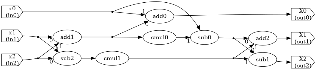
Display the SFG with l1-norm values for all signals
sfg.display(info="l1-norm")
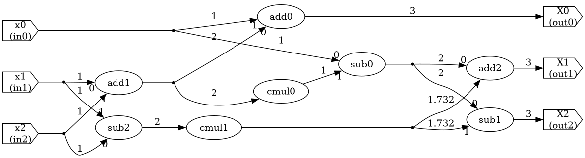
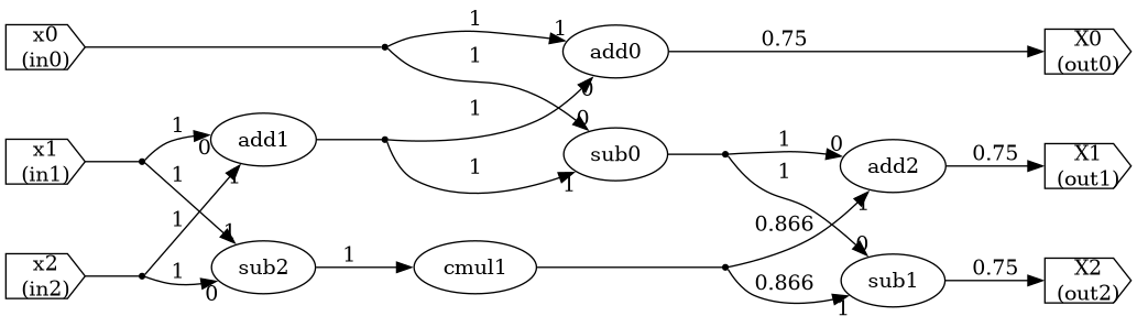
Introduce scaling such that the l1-norm values do not exceed 1 (safe-scaling)
sfg["add1"].out0_scale = 1
sfg["sub2"].out0_scale = 1
sfg["add0"].out0_scale = 1
sfg["add2"].out0_scale = 1
sfg["sub1"].out0_scale = 1

sfg["add0"].in1_scale = 1
sfg["sub0"].in0_scale = 1

sfg = sfg.remove_operation("cmul0")
sfg["sub0"].in0_scale = 0
sfg["sub0"].out0_scale = 1

sim1 = Simulation(sfg, data)
sim_res = sim1.run()
assert np.allclose(sim_res[0], fft_reference[0]/4, atol=1e-3)
assert np.allclose(sim_res[1], fft_reference[1]/4, atol=1e-3)
assert np.allclose(sim_res[2], fft_reference[2]/4, atol=1e-3)

sfg.display(info="l1-norm")
First we must define the latency and execution time for each type of operation
from b_asic.core_operations import Addition, Subtraction, ConstantMultiplication

sfg.set_latency_of_type(Addition, 1)
sfg.set_execution_time_of_type(Addition, 1)
sfg.set_latency_of_type(Subtraction, 1)
sfg.set_execution_time_of_type(Subtraction, 1)
sfg.set_latency_of_type(ConstantMultiplication, 2)
sfg.set_execution_time_of_type(ConstantMultiplication, 1)
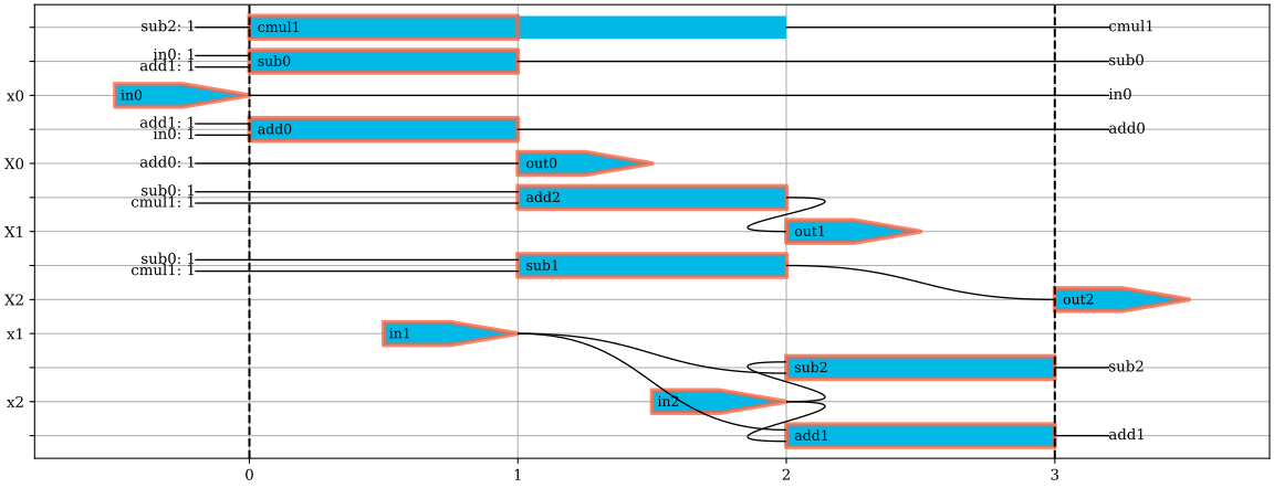
We want a streaming implementation using the minimal amount of operators, i.e. one parallel input and one parallel operation -> the operations should be distributed over three clock cycles.
Let us use a scheduling algorithm for that.
from b_asic import Schedule, HybridScheduler

# We need 1 PE of each type
resources={Addition: 1, Subtraction: 1, ConstantMultiplication: 1}
# Specify the input and output timing constraints
input_times = {f"in{i}": i for i in range(3)}
output_delta_times = {f"out{i}": i for i in range(3)}

scheduler = HybridScheduler(
    max_resources=resources,
    input_times=input_times,
    output_delta_times=output_delta_times,
)
# Schedule over three cycles, enable cyclic scheduling to allow wrapping around the schedule edge
schedule = Schedule(sfg, scheduler, schedule_time=3, cyclic=True)
schedule
Map to an architecture with the desired number of PEs and the minimal amount of memories and multiplexing.
from b_asic.resource_assigner import assign_processing_elements_and_memories
from b_asic.architecture import Architecture

# Automatic resource assignment
pes, mems, direct = assign_processing_elements_and_memories(
    schedule,
    strategy="ilp_min_mux",
    memory_read_ports=1,
    memory_write_ports=1,
    memory_total_ports=2,
    memory_type="RAM",
)
# Create an architecture and display it
arch = Architecture(pes, mems, "r3", direct)
arch
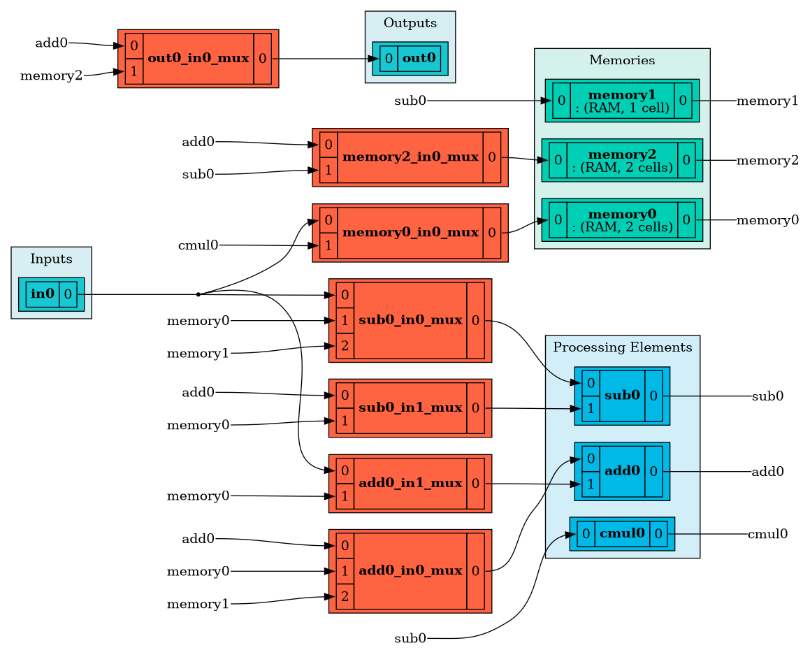
Generate VHDL for the created architecture.
from b_asic.data_type import DataType
from b_asic.code_printer import VhdlPrinter

# Use a fixed-point complex data type using 16 bits for each part
WL = 16
dt = DataType(WL, is_complex=True)

# Generate VHDL code for the architecture with registers on I/O ports
printer = VhdlPrinter(dt)
printer.print(arch, path="generated_separate", io_registers=True)
Simulate and generate a testbench for the design.
from b_asic.tb_printer import CocotbPrinter

# Generate N complex points within the unit disk
N = 1000
rng = np.random.default_rng()
step = 2**(-(WL - 1))
half = 2**(WL - 1)
def _rand_unit_disk(rng, n):
    out = []
    while len(out) < n:
        re = rng.integers(-half, half) * step
        im = rng.integers(-half, half) * step
        if re**2 + im**2 < 1:
            out.append(re + 1j * im)
    return out

data = [_rand_unit_disk(rng, N) for _ in range(3)]
# Run a simulation with the generated input data for N iterations
sim = Simulation(schedule.sfg, data, dt)
sim.run_for(N)

# Generate the testbench for the simulation results
tb_printer = CocotbPrinter(sim.results)
tb_printer.print(
    arch,
    schedule,
    path="generated_separate",
    simulator="questa", # can be set to any simulator that Cocotb supports, e.g. "ghdl" or "nvc"
    waves=True, # enable waveform generation
    io_registers=True, # specify that I/O ports have registers
)
Let us now model the algorithm using “AddSub” operations i.e. an operation that adds or subtracts based on a control signal.
from b_asic.core_operations import AddSub

sfg = sfg.rewrite(AddSub, Addition)
sfg = sfg.rewrite(AddSub, Subtraction)
sfg
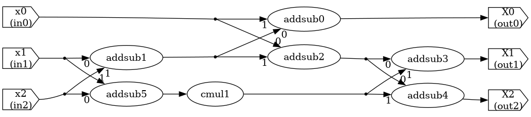
Do the same scheduling and mapping to an architecture again.
sfg.set_latency_of_type(AddSub, 1)
sfg.set_execution_time_of_type(AddSub, 1)

resources={AddSub: 2, ConstantMultiplication: 1}
scheduler = HybridScheduler(
    max_resources=resources,
    input_times=input_times,
    output_delta_times=output_delta_times,
)
schedule = Schedule(sfg, scheduler, schedule_time=3, cyclic=True)
schedule

pes, mems, direct = assign_processing_elements_and_memories(
    schedule,
    strategy="ilp_min_mux",
    memory_read_ports=1,
    memory_write_ports=1,
    memory_total_ports=2,
    memory_type="RAM",
)
arch = Architecture(pes, mems, "r3", direct)
arch
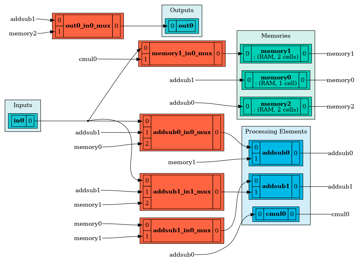
Generate VHDL and a testbench for the new architecture.
printer.print(arch, path="generated_addsub", io_registers=True)

sim = Simulation(schedule.sfg, data, dt)
sim.run_for(N)

tb_printer = CocotbPrinter(sim.results)
tb_printer.print(
    arch,
    schedule,
    path="generated_addsub",
    simulator="questa",
    waves=True,
    io_registers=True,
)
We can convert “cmul1” into addsubs with shifts on the inputs.
If we use 3 addsub PEs we have three addsub operations to spare on the constant multiplication, since the algorithm contains 6 addsub operations to compute over 3 cycles. 7095/8192 is the best approximation using three addsubs so let us use that one.
Factorize the constant multiplication into smaller parts. This is done since the CSD representation of these constants is optimal, which is not the case for 7095/8192.
Start by propagating the imaginary multiplication into the inputs of “addsub3” and “addsub4” as well as factoring the constant into two smaller parts and rewriting them into addsubs with shifts.
c310 = ConstantMultiplication(55/64)
c311 = ConstantMultiplication(129/128)

sfg = sfg.replace("cmul1", c310)
sfg = sfg.insert_operation_after("cmul0", c311)
sfg["addsub3"].mul_j = True
sfg["addsub4"].mul_j = True

sfg = sfg.rewrite(AddSub, ConstantMultiplication)

# Validate the modified SFG
data = [[rng.random() + 1j * rng.random()] for _ in range(3)]
fft_reference = np.fft.fft([d[0] for d in data])
sim1 = Simulation(sfg, data)
sim_res = sim1.run()
assert np.allclose(sim_res[0], fft_reference[0]/4, atol=1e-3)
assert np.allclose(sim_res[1], fft_reference[1]/4, atol=1e-3)
assert np.allclose(sim_res[2], fft_reference[2]/4, atol=1e-3)

sfg

Now we can proceed with scheduling and mapping to an architecture consisting of 3 addsub PEs, because we now have 9 addsub operations to compute over 3 cycles.
sfg.set_latency_of_type(AddSub, 1)
sfg.set_execution_time_of_type(AddSub, 1)

resources={AddSub: 3}
scheduler = HybridScheduler(
    max_resources=resources,
    input_times=input_times,
    output_delta_times=output_delta_times,
)
schedule = Schedule(sfg, scheduler, schedule_time=3, cyclic=True)
schedule

pes, mems, direct = assign_processing_elements_and_memories(
    schedule,
    strategy="ilp_min_mux",
    memory_read_ports=1,
    memory_write_ports=1,
    memory_total_ports=2,
    memory_type="RAM",
)
arch = Architecture(pes, mems, "r3", direct)
arch
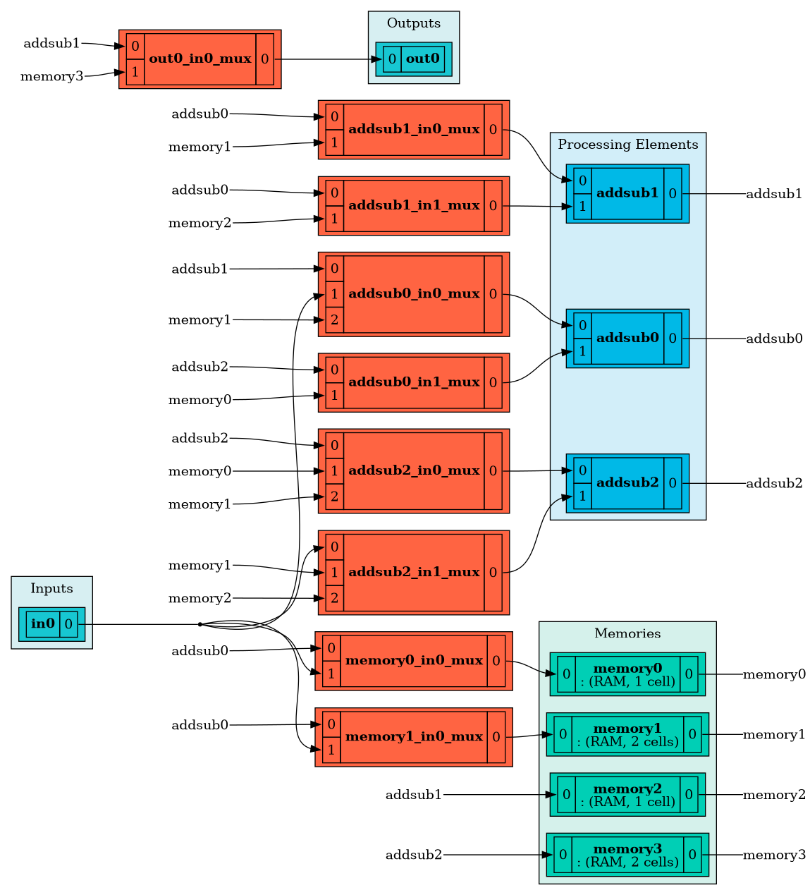
Generate VHDL and a testbench for the new architecture
printer.print(arch, path="generated_shiftandadd", io_registers=True)

data = [_rand_unit_disk(rng, N) for _ in range(3)]
sim = Simulation(schedule.sfg, data, dt)
sim.run_for(N)

tb_printer = CocotbPrinter(sim.results)
tb_printer.print(
    arch,
    schedule,
    path="generated_shiftandadd",
    simulator="questa",
    waves=True,
    io_registers=True,
)
Finally, by unfolding the schedule, the schedule can be further optimized due to increased flexibility.
sfg = sfg.unfold(2)
sfg.display()
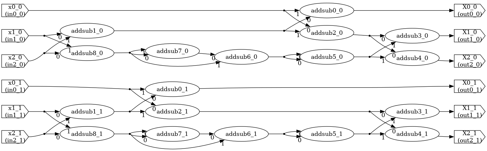
We then schedule the unfolded SFG, i.e. scheduling 2 iterations of the algorithm over 6 cycles.
from b_asic import Schedule, HybridScheduler, AddSub

sfg.set_latency_of_type(AddSub, 1)
sfg.set_execution_time_of_type(AddSub, 1)

resources={"addsub": 3}
input_times = {f"in{i}_0": i for i in range(3)}
input_times |= {f"in{i}_1": i+3 for i in range(3)}
output_delta_times = {f"out{i}_0": i for i in range(3)}
output_delta_times |= {f"out{i}_1": i+3 for i in range(3)}

scheduler = HybridScheduler(
    max_resources=resources,
    input_times=input_times,
    output_delta_times=output_delta_times,
)
schedule = Schedule(sfg, scheduler, schedule_time=6, cyclic=True)
schedule
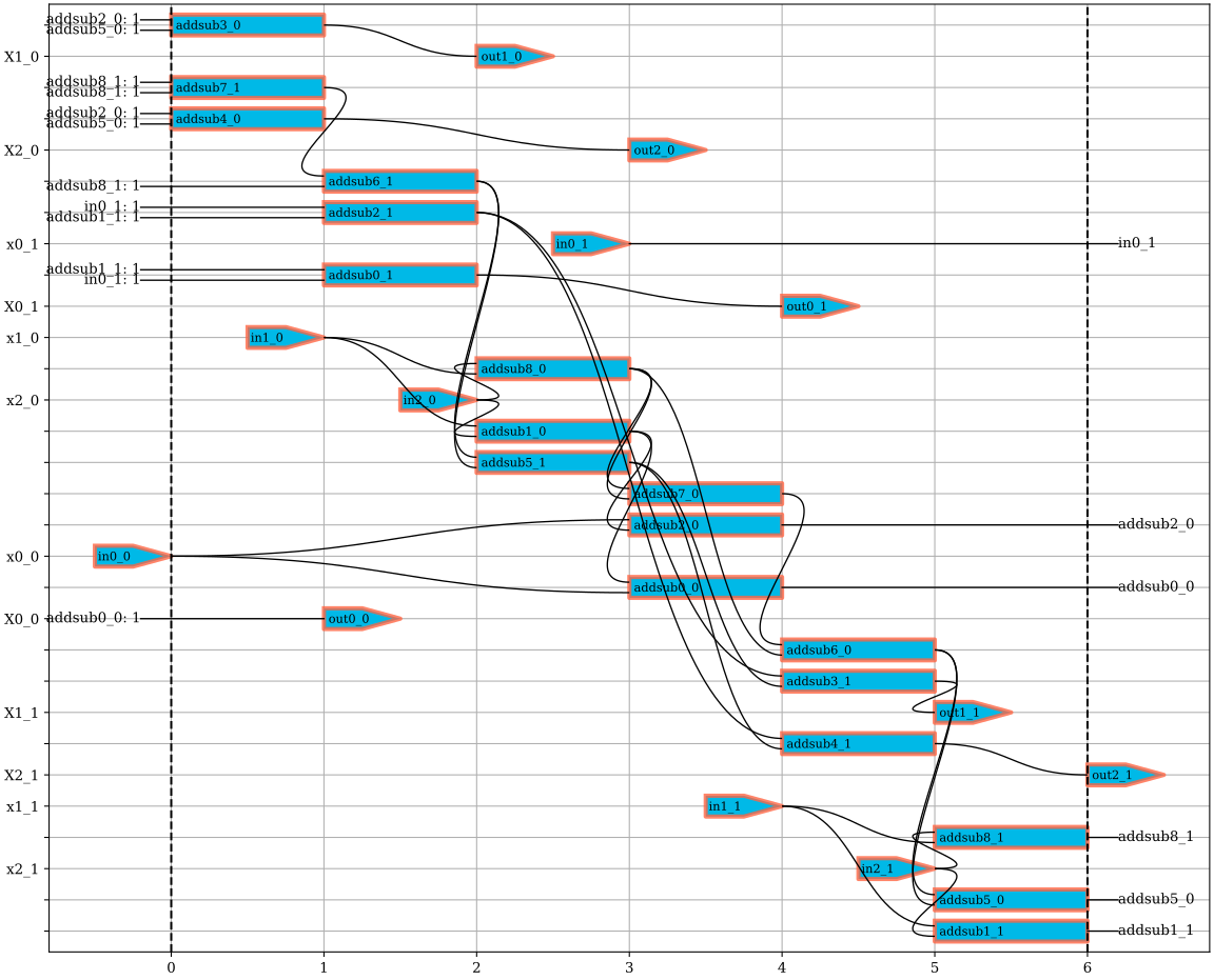
Manual schedule optimization, written out to the terminal when using the scheduling GUI, “schedule.edit()”. We achieve a schedule with a latency of one less clock cycle and reduce the number of concurrent reads/writes to memory. Thus we also expect this optimization to reduce the number of memories by one.
schedule.move_operation('addsub3_1', -1)
schedule.move_operation('out0_0', -1)
schedule.move_operation('out1_0', -1)
schedule.move_operation('out2_0', -1)
schedule.move_operation('out0_1', -1)
schedule.move_operation('out1_1', -1)
schedule.move_operation('out2_1', -1)
schedule.move_operation('addsub2_0', 1)
schedule.move_operation('addsub4_1', -1)
schedule.move_operation('addsub0_0', 1)
schedule
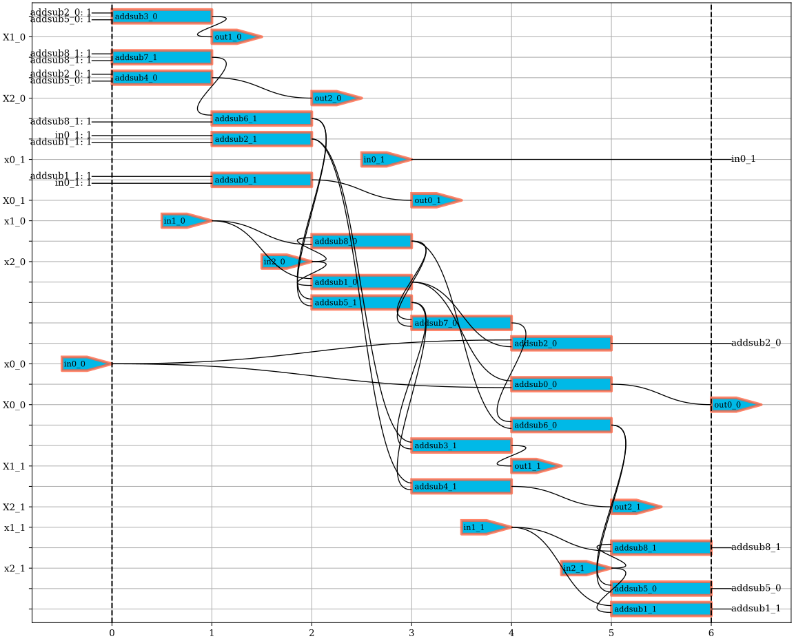
Generating an architecture for the optimized schedule.
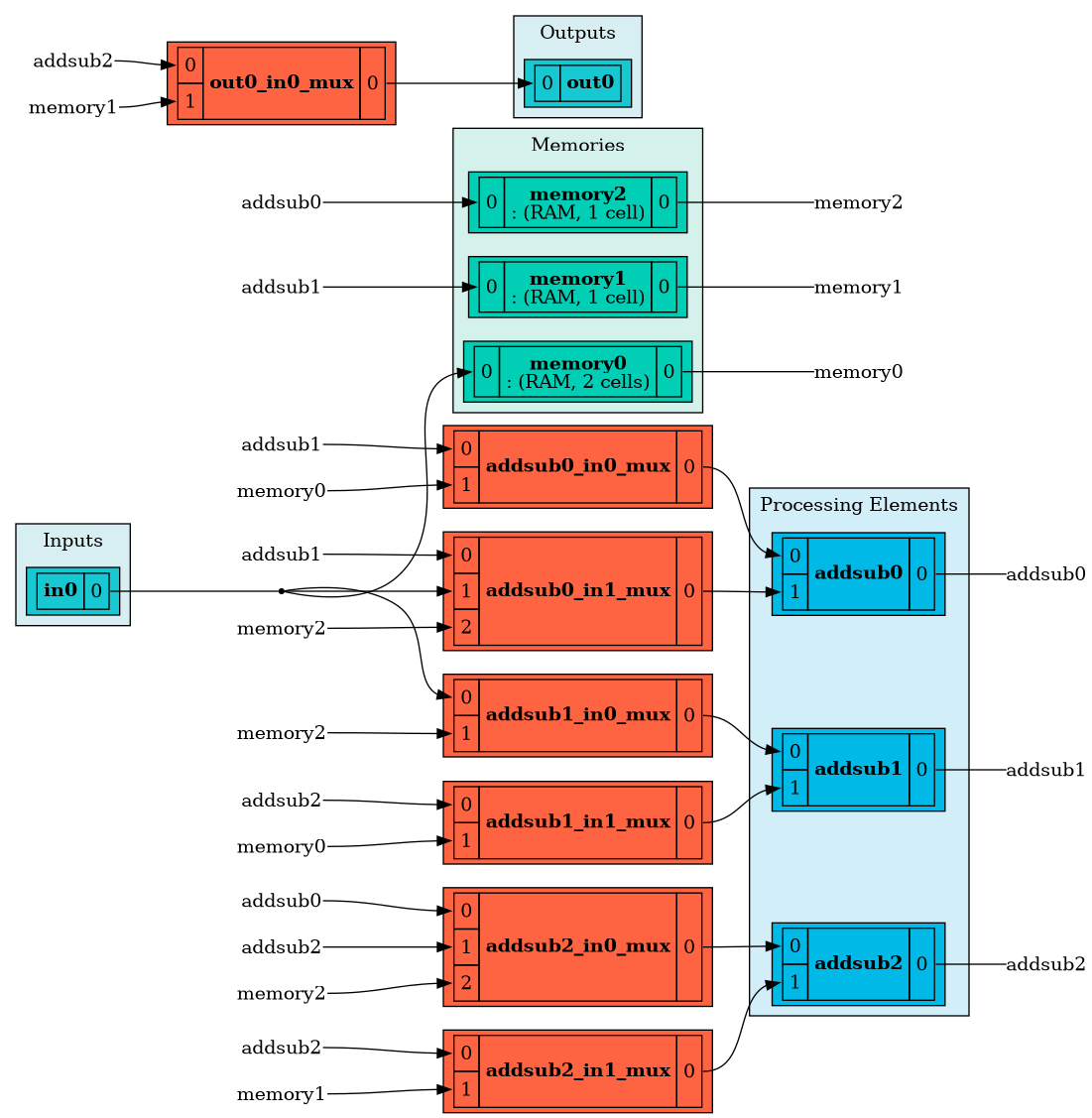
As seen, the architecture now only consists of three memories, which is an improvement compared to the previous one.
Finally, generate VHDL and a testbench for the optimized architecture.
printer.print(arch, path="generated_optimized", io_registers=True)

data = [_rand_unit_disk(rng, N) for _ in range(6)]
sim = Simulation(schedule.sfg, data, dt)
sim.run_for(N)

tb_printer = CocotbPrinter(sim.results)
tb_printer.print(
    arch,
    schedule,
    path="generated_optimized",
    simulator="questa",
    waves=True,
    io_registers=True,
)
Total running time of the script: (0 minutes 2.219 seconds)