Note
Go to the end to download the full example code.
Simulating a multi-rate filter
Build a rational sample-rate converter using Expansion and Compression around an FIR filter. Simulation handles the rate changes without modifying this SFG.
import numpy as np

from b_asic import SFG, Compression, Expansion, Input, Output, Simulation
from b_asic.sfg_generators import fir
Expand by three, filter at the higher rate, and compress by two.

Each period consumes two input samples and produces three output samples.
samples = np.array([1.0, -2.0, 3.0, 0.5, 2.0, -1.0])
simulation = Simulation(graph, [samples])
assert simulation.input_samples_per_iteration == (2,)
assert simulation.output_samples_per_iteration == (3,)
simulation.run()
converted = simulation.results[graph.output_operations[0].graph_id]

expanded = np.zeros(3 * len(samples))
expanded[::3] = samples
reference = np.convolve(expanded, coefficients)[: len(expanded) : 2]
np.testing.assert_allclose(converted, reference)
print("Multi-rate simulation matches zero insertion, FIR filtering, and compression.")
Multi-rate simulation matches zero insertion, FIR filtering, and compression.
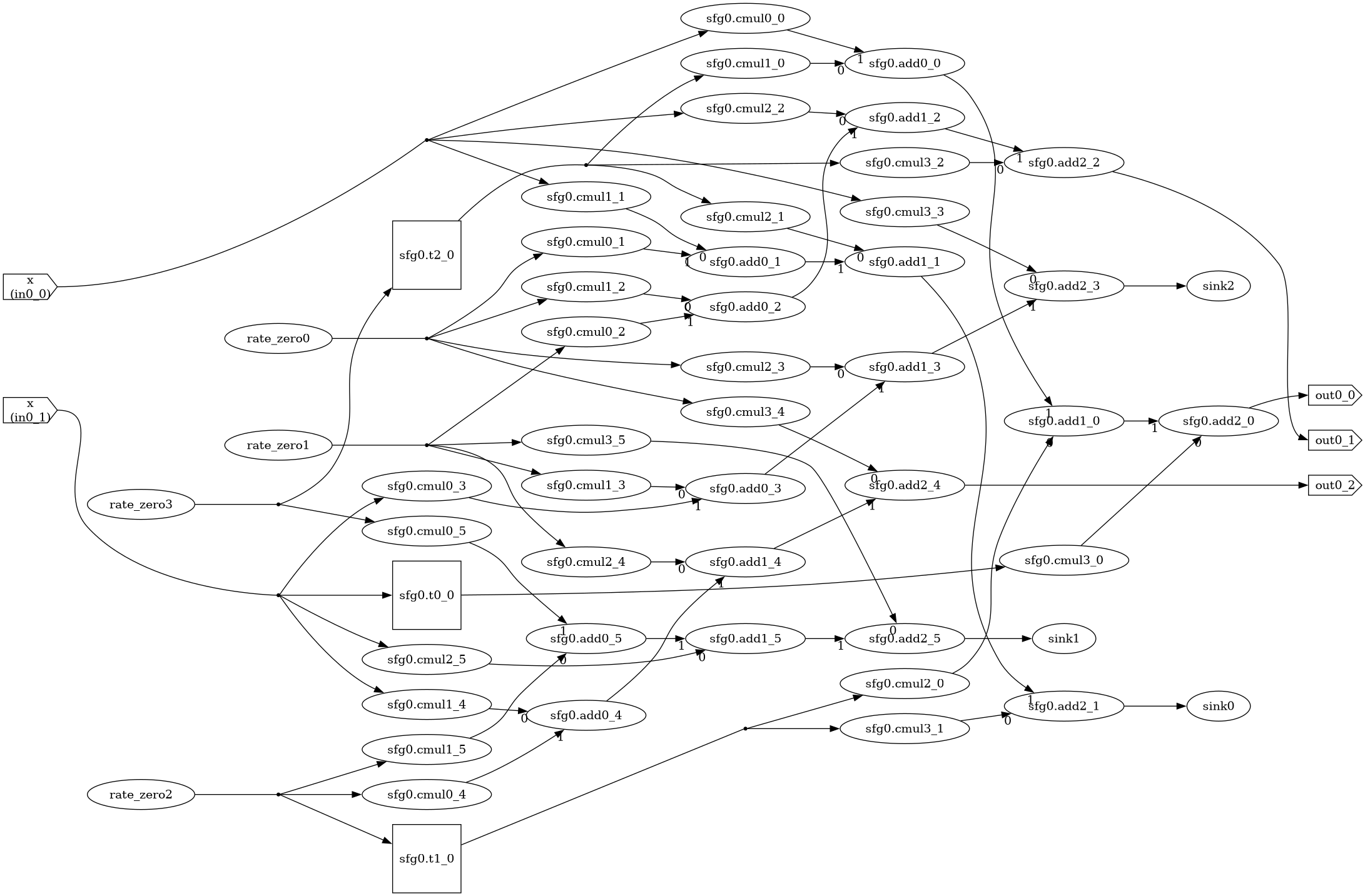
Obtain a single-rate phase graph explicitly for later architecture work.
normalization = graph.to_single_rate()
normalization.sfg  # noqa: B018
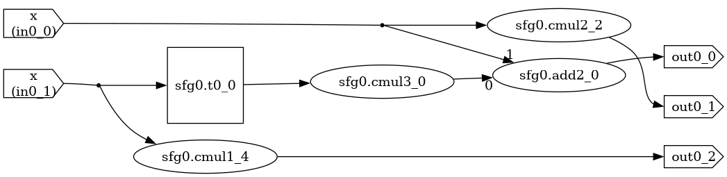
Simplification removes arithmetic on inserted zeros and unused output phases.
single_rate = normalization.sfg.constant_propagation().sink_propagation()
single_rate  # noqa: B018
Total running time of the script: (0 minutes 0.178 seconds)