Mapping to Hardware

When deriving a time-multiplexed implementation from an SFG, operations must be spread out in time in a way that respects the specifications and the dependencies between operations. This process is called scheduling, and has a significant impact on the resulting architecture, and thus, on the implementation results.

Scheduling

Schedules are represented by Schedule objects, and can be derived using a Scheduler, or manually. Continuing with a simplified version of the WDF from the previous tutorial (unscaled).

from scipy.signal import iirfilter
from b_asic.sfg_generators.wave_digital_filters import lattice_wdf
from b_asic.wdf import lattice_coeffs_from_tf
from b_asic.quantization import quantize

b, a = iirfilter(N=7, Wn=0.3, rp=0.1, rs=60, btype="low", ftype="ellip")
adaptor_coeffs = lattice_coeffs_from_tf(a)
quantized_coeffs = [quantize(c, fractional_bits=14) for c in adaptor_coeffs]

wdf_sfg = lattice_wdf(quantized_coeffs)
wdf_sfg

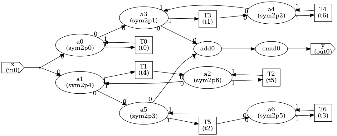
One can employ a “trick” to use an adaptor for the addition and multiplication with 0.5.

wdf_sfg = lattice_wdf(quantized_coeffs, only_adaptors=True)
wdf_sfg

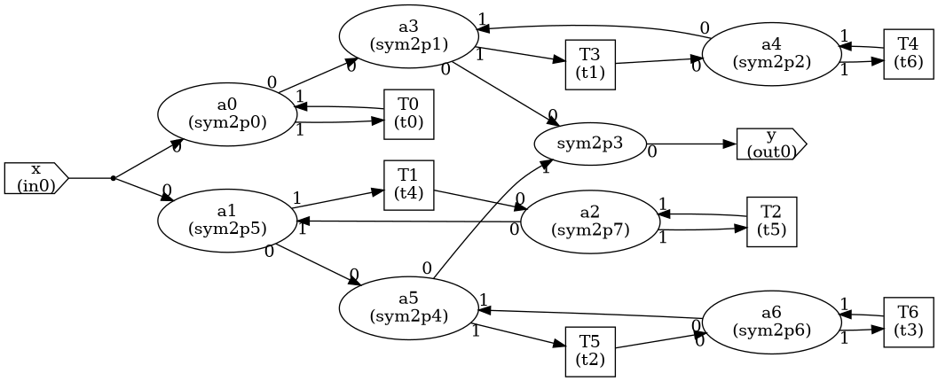
This is a good idea since it means all operations are of the same type, and can later be mapped to the same type of processing elements (PEs).

Before scheduling, latencies and execution times (initiation intervals) of the operations must be set. We want to use “fully” pipelined adaptors, so we set the latencies to four and the execution times to one.

from b_asic.wdf_operations import SymmetricTwoportAdaptor

wdf_sfg.set_latency_of_type(SymmetricTwoportAdaptor, 4)
wdf_sfg.set_execution_time_of_type(SymmetricTwoportAdaptor, 1)

From this SFG, an initial schedule can be derived

from b_asic.schedule import Schedule

schedule = Schedule(wdf_sfg)
schedule

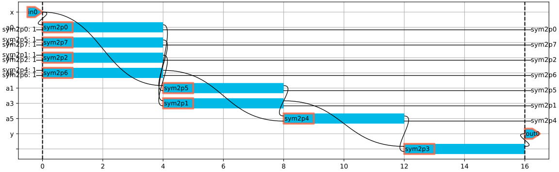
Operations with concurrent execution times, (i.e. are started at the same time) must be implemented on different PEs. Thus, the initial schedule requires 4 PEs. By enabling cyclic scheduling and moving operations, a schedule with a shorter scheduling period using one adaptor can be derived.

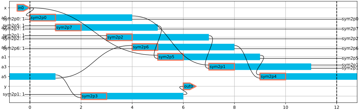
For example, if the data rate is 20 MHz, and have access to an FPGA with a clock frequency of 240 MHz, we can target a schedule period of 12 cycles and thus spread the operations out such that we only use two adaptor processing element. This is done through edit(), the scheduling steps are output to the terminal, and we use these to reproduce the manual scheduling steps.

schedule = Schedule(wdf_sfg, cyclic=True)
schedule.move_operation('out0', 9)
schedule.move_operation('sym2p3', 4)
schedule.move_operation('sym2p3', 5)
schedule.move_operation('sym2p4', 1)
schedule.move_operation('sym2p6', 4)
schedule.move_operation('sym2p4', 7)
schedule.move_operation('sym2p1', 1)
schedule.set_schedule_time(12)
schedule.move_operation('sym2p1', 1)
schedule.move_operation('sym2p6', 1)
schedule.move_operation('sym2p5', 2)
schedule.move_operation('sym2p2', 2)
schedule.move_operation('sym2p7', 1)
schedule.move_operation('sym2p6', -1)
schedule.move_operation('sym2p4', -2)
schedule.move_operation('sym2p5', -1)
schedule.move_operation('sym2p4', -1)
schedule.move_operation('sym2p3', -4)
schedule.move_operation('sym2p6', -1)
schedule.move_operation('out0', -4)
schedule.move_operation('sym2p1', 1)
schedule.move_operation('sym2p2', 1)
schedule.move_operation('sym2p6', 1)
schedule.move_y_location('sym2p3', 9, True)
schedule.move_operation('out0', 1)
schedule.move_operation('sym2p3', 1)
schedule.move_operation('sym2p4', 1)
schedule.move_operation('sym2p4', -1)
schedule.move_operation('sym2p6', -3)
schedule.move_operation('sym2p6', 3)
schedule.move_operation('sym2p6', -2)
schedule.move_y_location('sym2p6', 3, True)
schedule.move_operation('sym2p6', 2)
schedule.move_y_location('sym2p6', 5, True)
schedule

Resource Assignment

The next step will be to handle intermediate results as memory variables and to derive a hardware architecture.

variables = schedule.get_memory_variables()
variables

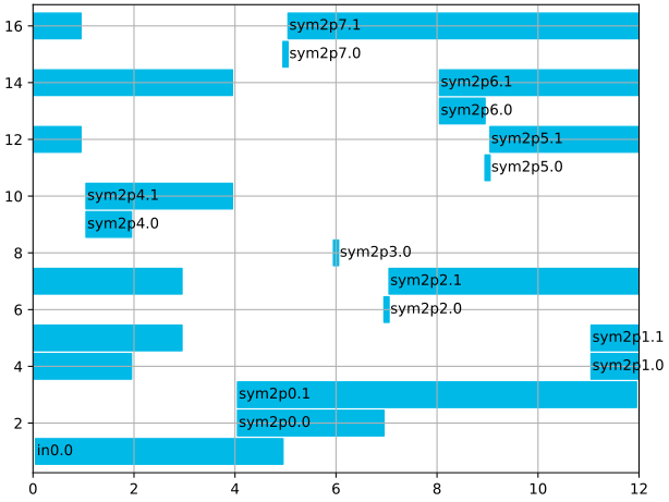
Direct variables (ones with lifetime of zero) can be passed directly

direct, variables = variables.split_on_length()

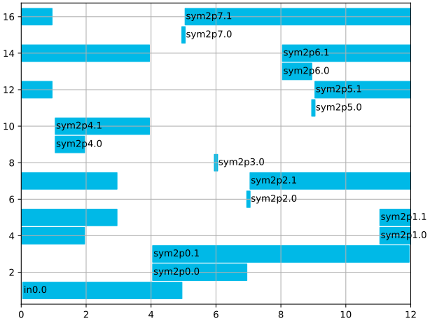
Assuming dual-port (one read, one write) memories, variables can share memory if they are not written to or read from at the same time step.

variable_groups = variables.split_on_ports(
    write_ports=1,
    read_ports=1,
    total_ports=2,
)

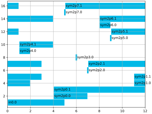
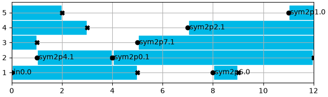
In this case, we have two overlapping accesses, can you see where? Thus we need two memories. Memory 0 has the following variables assigned

variable_groups[0]

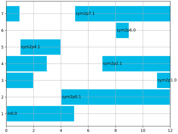
The last remaining step of memory 0 is to assign the variables to cells in the memory

from b_asic.architecture import Memory
mem0 = Memory(variable_groups[0], assign=True, entity_name="m0")
mem0.content

Memory 1 has the following variables assigned

variable_groups[1]

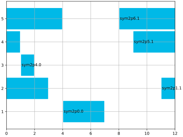
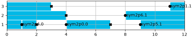
The last remaining step of memory 1

mem1 = Memory(variable_groups[1], assign=True, entity_name="m1")
mem1.content

Before an architecture can be derived, operations and I/O must be assigned to resources.

from b_asic.special_operations import Input, Output
from b_asic.architecture import ProcessingElement

ops = schedule.get_operations()
adaptor_ops = ops.get_by_type(SymmetricTwoportAdaptor)
adaptor = ProcessingElement(adaptor_ops, entity_name="a")
input_ops = ops.get_by_type(Input)
input_pe = ProcessingElement(input_ops, entity_name="x")
output_ops = ops.get_by_type(Output)
output_pe = ProcessingElement(output_ops, entity_name="y")

Now we can derive an architecture, and render it.

from b_asic.architecture import Architecture

arch = Architecture(
    processing_elements=[adaptor, input_pe, output_pe],
    memories=[mem0, mem1],
    direct_interconnects=direct,
    entity_name="wdf",
)
arch

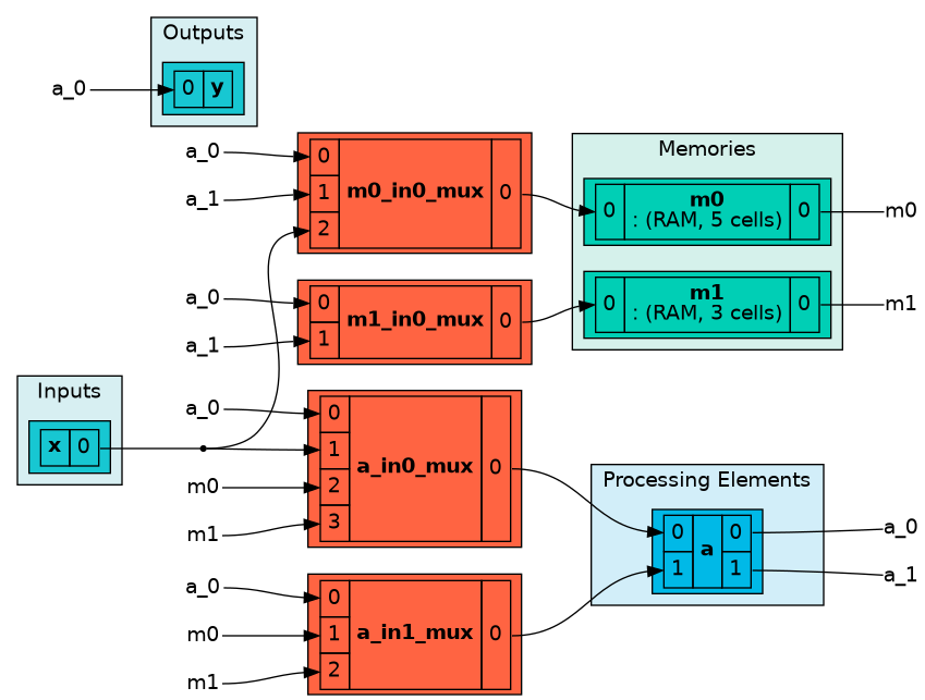
Here, the red boxes represent multiplexers, which are needed a port gets its data from multiple sources, depending on the schedule. Interestingly, both input ports to the adaptor get their data from both memories. This is uneccecary and leads to bigger multiplexers. There are several ways to derive an architectures with smaller multiplexers. One can, reschedule, move variables between memories, or use a smarter resource assignment algorithm. However, for this tutorial, we are satisfied, and can move on to generate HDL describing this architecture, along with a testbench for validation.