Simulation

Finite-wordlength analysis is a critical step in the design of algorithms. Unfortunately, is is often overlooked or oversimplified due to the complexity of the analysis. With B-ASIC, a correct analysis becomes easier.

SFGs can be simulated in arbitrary precision using Simulation and DataType. This tutorial showcases this through a finite-wordlength analysis of a wave digital filter.

Algorithm

We begin by designing an elliptic low-pass filter with the following specifications:

• Order: 7

• Passband edge frequency: 0.3 times the Nyquist frequency

• Passband ripple: 0.1 dB

• Stopband attenuation: 60 dB

from scipy.signal import iirfilter

from b_asic.wdf import lattice_coeffs_from_tf

b, a = iirfilter(N=7, Wn=0.3, rp=0.1, rs=60, btype="low", ftype="ellip")

print("Transfer function coefficients:")
print("Numerator:", b)
print("Denominator:", a)

Transfer function coefficients:
Numerator: [0.00698396 0.00219871 0.0142081  0.01065808 0.01065808 0.0142081
 0.00219871 0.00698396]
Denominator: [ 1.         -3.97699108  7.99282358 -9.90310426  8.08290621 -4.30338914
  1.38344285 -0.20759045]

We then use the module b_asic.wdf to derive adaptor coefficients for a lattice structure that implements the filter.

adaptor_coeffs = lattice_coeffs_from_tf(a)
print("Lattice adaptor coefficients:")
for i, coeff in enumerate(adaptor_coeffs):
    print(f"    a{i}: {coeff}")

Lattice adaptor coefficients:
    a0: 0.6072682339178634
    a1: -0.9233304755403088
    a2: 0.5683222541662454
    a3: -0.7388670919448468
    a4: 0.635533951021361
    a5: -0.5010756697748922
    a6: 0.7804684909217103

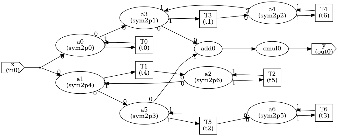
Now, use an SFG generator to construct the SFG of the lattice wave digital filter.

from b_asic.sfg_generators.wave_digital_filters import lattice_wdf

wdf_sfg = lattice_wdf(adaptor_coeffs)
wdf_sfg

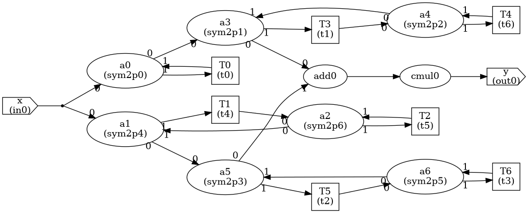
Here, each adaptor is represented as a single operation with the following equations:

\[\begin{split}y_0 & = x_1 + \alpha\times\left(x_1 - x_0\right)\\ y_1 & = x_0 + \alpha\times\left(x_1 - x_0\right)\end{split}\]

where \(\alpha\) is the adaptor coefficient. The coefficients for the adaptors are now represented as 64-bit floating point numbers. Multiplication with such a coefficient will be extremely expensive in terms of hardware resources. As such, we want to quantize the coefficients, as much as possible. But before we do that, we need to investigate the need for scaling the coefficients.

Coefficient Quantization

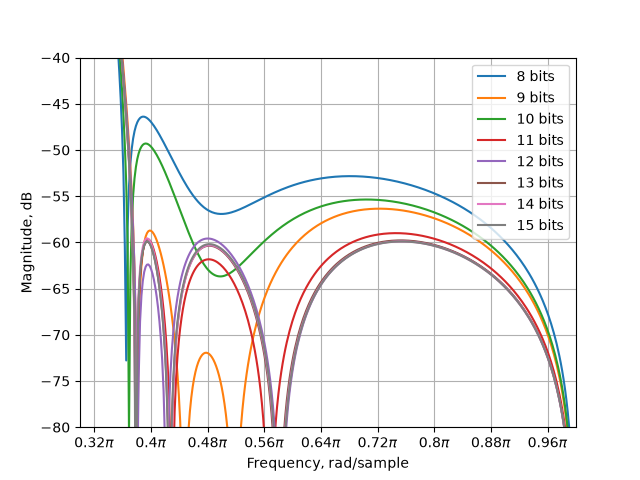
Coefficient quantization introduces a static error to the transfer function. In order to investigate the effects of quantization, we quantize the coefficients to 5 to 11 fractional bits, and derive the transfer functions of the resulting filters.

import matplotlib.pyplot as plt
import numpy as np
from scipy.signal import chirp, freqz

from b_asic.quantization import quantize
from b_asic.signal_generator import Impulse
from b_asic.simulation import Simulation

w_ref, H_ref = freqz(b, a)

impulse_responses = {}
sfgs = {}
for n_bits in range(8, 16):
    q_coeffs = [quantize(c, fractional_bits=n_bits) for c in adaptor_coeffs]
    sfg = wdf_sfg.copy()
    for i in range(len(q_coeffs)):
        sfg.find_by_name(f"a{i}")[0].value = q_coeffs[i]
    sfgs[n_bits] = sfg

    sim = Simulation(sfg, [Impulse()])
    sim.run_for(1_000)
    impulse_responses[n_bits] = np.array([float(v) for v in sim.results["out0"]])

Stopband attenuation plotted for different wordlengths.

from mplsignal import freqz_fir

fig, ax = plt.subplots()
for n_bits, h in impulse_responses.items():
    freqz_fir(h, ax=ax, style="magnitude", label=f"{n_bits} bits")

ax.legend()
ax.set_xlim(0.3 * np.pi)
ax.set_ylim(-80, -40)
ax.grid(True)

Passband attenuation plotted for different wordlengths.

fig, ax = plt.subplots()
for n_bits, h in impulse_responses.items():
    freqz_fir(h, ax=ax, style="magnitude", label=f"{n_bits} bits")

ax.legend()
ax.set_xlim(0, 0.32 * np.pi)
ax.set_ylim(-0.15, 0.05)
ax.grid(True)

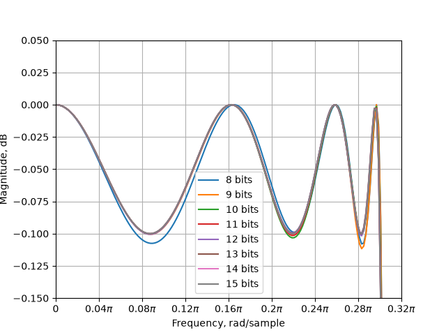
As a conclusion, one can see that coefficient quantization leeds to a similar but different algorithm. We can now choose a number of bits that we deem to meet our specification. In this case, let us continue with 14 bits as this meets the stopband attenuation requirement of 60 dB.

q_sfg = sfgs[14]

Scaling

As implementation will be done in fixed-point arithmetic, thus, we need to investigate the need for scaling to maximize the dynamic range of the filter and protect against overflow. To investigate this, we can once again render the SFG, this time with the l2-norm values of all signals.

from b_asic.core_operations import LeftShift, RightShift
q_sfg.sfg_digraph(signal_info="l1-norm")

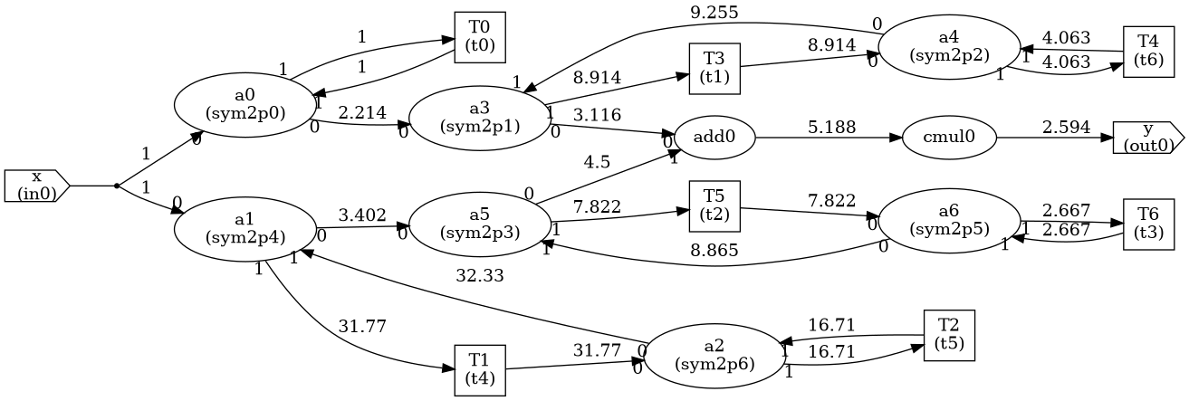
From the figure, we see that the l1-norm exceeds 1 at a lot of places, meaining that overflow can occur if we do not scale the input, which we want to prevent in this example. Note that one cannot scale inside loops…

Inserting appropriate shifts to safe-scale.

q_sfg = q_sfg.insert_operation_before("a0", RightShift(2), 0)
q_sfg = q_sfg.insert_operation_before("a1", RightShift(5), 0)
q_sfg = q_sfg.insert_operation_after("a0", RightShift(2), 0)
q_sfg = q_sfg.insert_operation_after("a3", LeftShift(1), 0)
q_sfg = q_sfg.insert_operation_after("a5", LeftShift(2), 0)
q_sfg = q_sfg.remove_operation("cmul0")
q_sfg.sfg_digraph(signal_info="l1-norm")

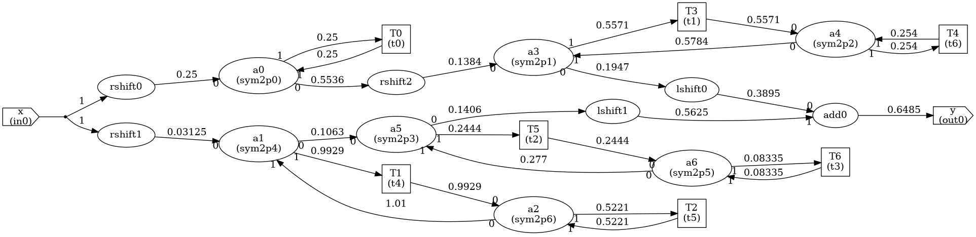
Note that the output is scaled by 1/4 now. However, it is not a problem since its just a matter of selecting the correct bits.

SNR Analysis

SNR is calculated as the ratio of the signal power to the noise power, where the noise is the difference between simulated outputs with and without quantization. This is calculated for a range of wordlengths along with magnitude truncation for data quantization, as it protects against limit-cycles while still being simple to implement.

from b_asic.data_type import DataType
from b_asic.quantization import QuantizationMode

N = 1_000
rng = np.random.default_rng(0)
wl_range = range(8, 19)
snr_values = []
for WL in wl_range:
    data = rng.integers(-2**(WL - 1), 2**(WL - 1), size=(1, N)) * 2**(-(WL - 1))
    dt = DataType(
        (1, WL),
        quantization_mode=QuantizationMode.MAGNITUDE_TRUNCATION
    )
    sim_quant = Simulation(q_sfg, data, data_type=dt)
    sim_quant.run_for(N)

    sim_ref = Simulation(q_sfg, data)
    sim_ref.run_for(N)

    out_ref = np.array([float(v) for v in sim_ref.results["out0"]])
    out_quant = np.array([float(v) for v in sim_quant.results["out0"]])

    P_signal = np.mean(out_ref**2)
    P_noise = np.mean((out_quant - out_ref) ** 2)
    snr_values.append(10 * np.log10(P_signal / P_noise))

fig, ax = plt.subplots()
ax.plot(wl_range, snr_values, marker="o")
ax.set_xlabel("Fractional bits")
ax.set_ylabel("SNR, dB")
ax.grid(True)

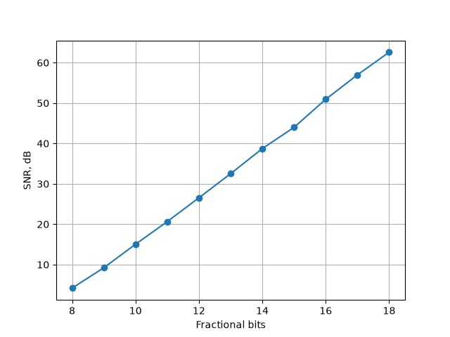
As expected from theory, the SNR increases linearly with the number of bits, with a slope of approximately 6 dB per bit. Here, one should simply pick a number of bits that meets the SNR requirements posed by the application. Note that if we had more information about the input data, there may exist a scaling that yields a better SNR. Since we have no such information, we safe-scale.

Conclusion

In this tutorial, we have seen how B-ASIC can be used to perform finite-wordlength analysis of algorithms targeting arbitrary precision. We are now ready to move on to the next step of the design process.