LTI System Analysis

In this example the state-space, transfer function, zero-pole-gain, and magnitude response for an LTI system are derived and visualized.

Signal-flow graph

6th-order elliptic low-pass filter

from b_asic.sfg_generators.digital_filters import direct_form_2_iir

b = [
    0.00688044, 0.00271194, 0.01334486, 0.00694836,
    0.01334486,0.00271194, 0.00688044
]
a = [
    1, -3.82875342, 7.15331101, -7.94817034,
    5.49500754, -2.23261844,  0.42049185
]

sfg = direct_form_2_iir(b, a)
sfg

State-space representation

ss = sfg.to_ss()
print(ss)

StateSpace (6 states, 1 inputs, 1 outputs)
  A = [[ 3.82875342, -7.15331101,  7.94817034, -5.49500754,  2.23261844,
  -0.42049185],
 [ 1.        ,  0.        ,  0.        ,  0.        ,  0.        ,
   0.        ],
 [ 0.        ,  1.        ,  0.        ,  0.        ,  0.        ,
   0.        ],
 [ 0.        ,  0.        ,  1.        ,  0.        ,  0.        ,
   0.        ],
 [ 0.        ,  0.        ,  0.        ,  1.        ,  0.        ,
   0.        ],
 [ 0.        ,  0.        ,  0.        ,  0.        ,  1.        ,
   0.        ]],
  B = [[1.],
 [0.],
 [0.],
 [0.],
 [0.],
 [0.]],
  C = [[ 0.02905545, -0.03587307,  0.06163527, -0.02446321,  0.01807334,
   0.00398727]],
  D = [[0.00688044]]

Transfer function

tf = sfg.to_tf()
print(tf)

TransferFunction (1 inputs, 1 outputs)
  Denominator: [ 1.         -3.82875342  7.15331101 -7.94817034  5.49500754 -2.23261844
  0.42049185]
  in0 Numerator: [0.00688044 0.00271194 0.01334486 0.00694836 0.01334486 0.00271194
 0.00688044]

Zero-pole-gain

zpk = sfg.to_zpk()
zeros, poles, gain = zpk["in0"]
print("Zeros:", zeros)
print("Poles:", poles)
print("Gain:", gain)

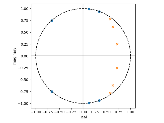
Zeros: [-0.66130483+0.75011727j -0.66130483-0.75011727j  0.34164245+0.93983j
  0.34164245-0.93983j     0.12258632+0.99245786j  0.12258632-0.99245786j]
Poles: [0.57014161+0.78145237j 0.57014161-0.78145237j 0.62440867+0.61818949j
 0.62440867-0.61818949j 0.71982644+0.25279698j 0.71982644-0.25279698j]
Gain: 0.006880439999999988

Pole-zero plot

import numpy as np
import matplotlib.pyplot as plt

theta = np.linspace(0, 2 * np.pi, 1024)

fig, ax = plt.subplots()
ax.plot(np.cos(theta), np.sin(theta), "k--")
ax.scatter(zeros.real, zeros.imag, marker="o")
ax.scatter(poles.real, poles.imag, marker="x")
ax.axhline(0, color="black")
ax.axvline(0, color="black")
ax.set_aspect("equal")
ax.set_xlabel("Real")
ax.set_ylabel("Imaginary")
plt.tight_layout()
plt.show()

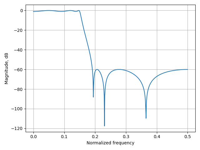
Magnitude response

from b_asic.signal_generator import Impulse
from b_asic.simulation import Simulation

sim = Simulation(sfg, [Impulse()])
sim.run_for(1024)

h = np.array(sim.results["out0"])

H = np.fft.rfft(h)
freqs = np.fft.rfftfreq(len(h))

fig, ax = plt.subplots()
ax.plot(freqs, 20 * np.log10(np.abs(H)))
ax.set_xlabel("Normalized frequency")
ax.set_ylabel("Magnitude, dB")
ax.grid(True)
plt.tight_layout()
plt.show()