Scheduling and Pipelining/Retiming

When scheduling cyclically (modulo) there is implicit pipelining/retiming taking place. B-ASIC can easily be used to showcase this.

import matplotlib.pyplot as plt
import numpy as np
from scipy import signal

from b_asic.core_operations import Addition, ConstantMultiplication
from b_asic.schedule import Schedule
from b_asic.scheduler import ALAPScheduler
from b_asic.sfg_generators import direct_form_1_iir
from b_asic.signal_generator import Impulse
from b_asic.simulation import Simulation

Design a simple direct form IIR low-pass filter.

N = 3
Wc = 0.2
b, a = signal.butter(N, Wc, btype="lowpass", output="ba")

Generate the corresponding signal-flow-graph (SFG).

sfg = direct_form_1_iir(b, a)
sfg

Set latencies and execution times of the operations.

sfg.set_latency_of_type(Addition, 1)
sfg.set_latency_of_type(ConstantMultiplication, 3)
sfg.set_execution_time_of_type(Addition, 1)
sfg.set_execution_time_of_type(ConstantMultiplication, 1)

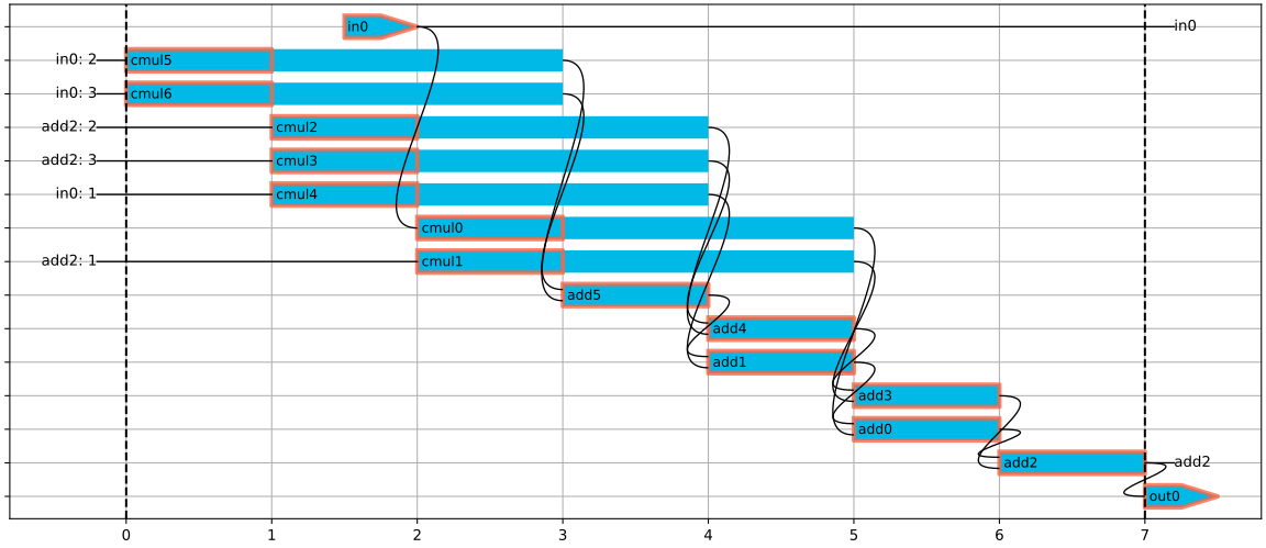
Print the critical path Tcp and the iteration period bound Tmin.

T_cp = sfg.critical_path_time()
print("Tcp:", T_cp)
T_min = sfg.iteration_period_bound()
print("Tmin:", T_min)

Tcp: 7
Tmin: 5

Create an ALAP schedule

schedule = Schedule(sfg, scheduler=ALAPScheduler(), cyclic=True)
schedule

Move some operations “over the edge” in order to reach Tcp = Tmin.

schedule.move_operation('out0', 2)
schedule.move_operation('add2', 2)
schedule.move_operation('add0', 2)
schedule.move_operation('add3', 2)
schedule.set_schedule_time(5)
schedule

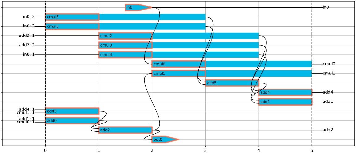
Print the new critical path Tcp that is now equal to Tmin.

T_cp = schedule.sfg.critical_path_time()
print("Tcp:", T_cp)
T_min = schedule.sfg.iteration_period_bound()
print("Tmin:", T_min)

Tcp: 5
Tmin: 5

Show the reconstructed SFG that is now pipelined/retimed compared to the original.

schedule.sfg

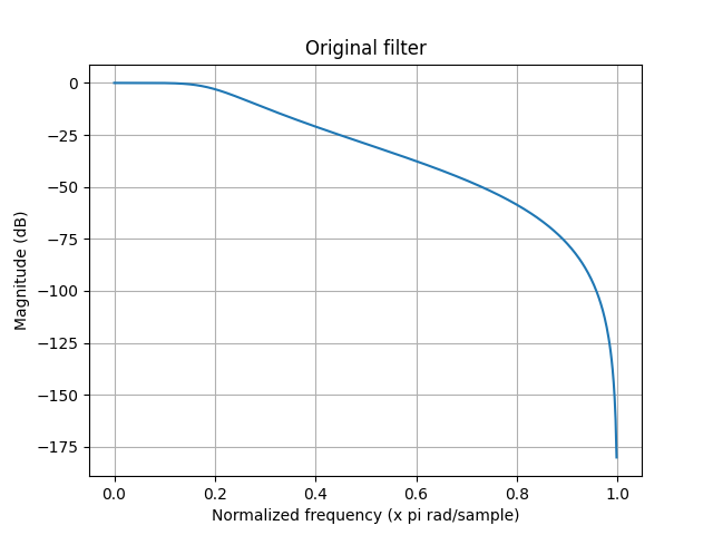
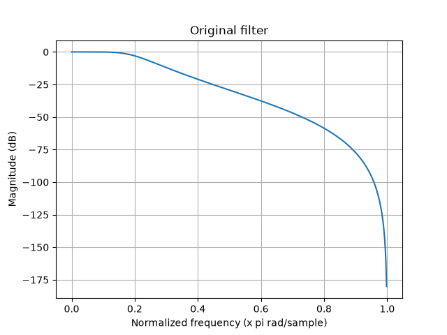
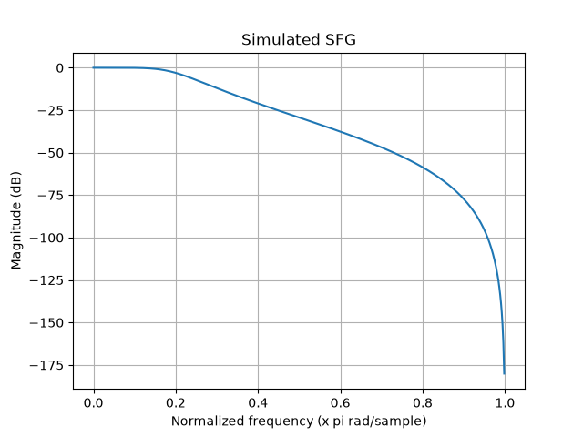
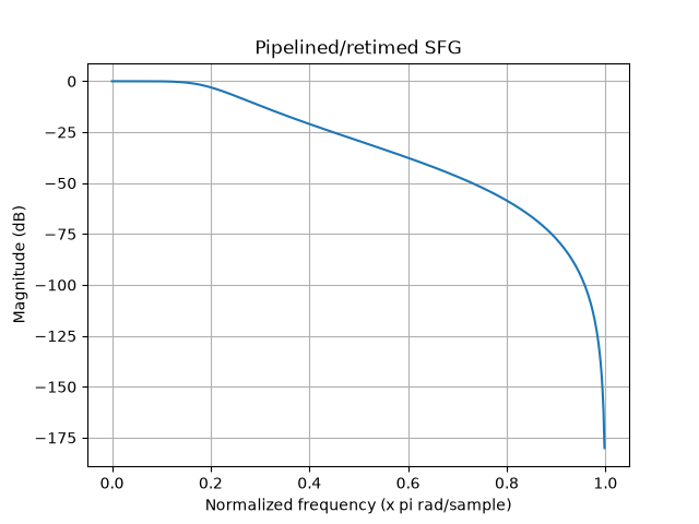
Simulate the impulse response of the original and reconstructed SFGs. Plot the frequency responses of the original filter, the original SFG and the reconstructed SFG to verify that the schedule is valid.

sim1 = Simulation(sfg, [Impulse()])
sim1.run_for(1000)

sim2 = Simulation(schedule.sfg, [Impulse()])
sim2.run_for(1000)

w, h = signal.freqz(b, a)

# Plot 1: Original filter
spectrum_0 = 20 * np.log10(np.abs(h))
plt.figure()
plt.plot(w / np.pi, spectrum_0)
plt.title("Original filter")
plt.xlabel("Normalized frequency (x pi rad/sample)")
plt.ylabel("Magnitude (dB)")
plt.grid(True)
plt.show()

# Plot 2: Simulated SFG
spectrum_1 = 20 * np.log10(np.abs(signal.freqz(sim1.results["out0"])[1]))
plt.figure()
plt.plot(w / np.pi, spectrum_1)
plt.title("Simulated SFG")
plt.xlabel("Normalized frequency (x pi rad/sample)")
plt.ylabel("Magnitude (dB)")
plt.grid(True)
plt.show()

# Plot 3: Recreated SFG
spectrum_2 = 20 * np.log10(np.abs(signal.freqz(sim2.results["out0"])[1]))
plt.figure()
plt.plot(w / np.pi, spectrum_2)
plt.title("Pipelined/retimed SFG")
plt.xlabel("Normalized frequency (x pi rad/sample)")
plt.ylabel("Magnitude (dB)")
plt.grid(True)
plt.show()

• 
• 
•